STEP 1: Activate "Developer" tab
Go on File - Options - Customize Ribbon - Select the "Developer" check box - OK: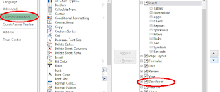
STEP 2: Add a group box
Go on Developer - Insert - Group box in Form Control: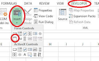
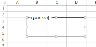
Then draw the group box and delete the text on it or write your question there:
STEP 3: Add option buttons
Go on Developer - Insert - Option button in Form Control: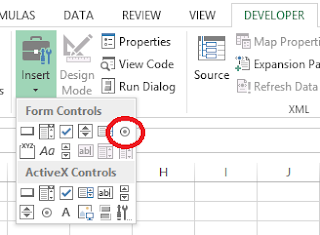
Then draw the option button COMPLETELY INSIDE the group box. This is very important, as if you don't draw it completely inside the group box, it will not be associated with other candidate answers of the same question and will not work properly. It's OK to move it outside of the group box afterwards but not before you draw it inside. Delete the text on the option button or write the candidate answer there:
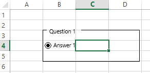
STEP 4: Complete the test
Repeat steps 3 and 2 as needed. If you need to reposition the form elements you first right click on them and then they are movable. Don't worry about accidentally selecting an option button; just make sure that checking an option button in a control group will not affect other control groups. If this happens then it is because the option buttons are not associated with the control group, because they were not drawn inside it, and you will have to draw a new one instead of it.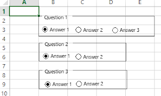
STEP 5: Automatically check the answers
Right click on the option buttons - Format Control - Set Cell link to a particular cell: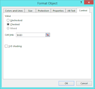
You only need to set one of the option buttons for each question. Make sure that option buttons of different questions all use different cell links. While you're in the Format Control window you can unset any accidentally set option buttons.
You now have the linked cell of each question contain a number which indicates the selected answer:
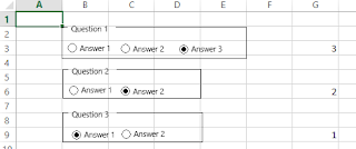
The number depends on the order in which the option buttons were added. Next write the correct answer next to each linked cell and next to that add a formula which checks if the right answer was selected. The formula is "=G3=H3" where "G3" is the linked cell and "H3" is the cell with the right answer.
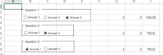
The 3 columns on the side show the chosen answer (automatically set by the option buttons), the correct answer (entered by you), and whether the right answer was chosen or not (automatically set by a formula which compares the previous two).
STEP 6: Automatically compute the mark
Finally, add the following formula under the TRUE/FALSE cells: "=COUNTIF(I3:I9,TRUE)" where "I3:I9" is the range of cells which are TRUE/FALSE.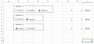
STEP 7: Barricade the Excel sheet
At the moment the answers are in plain sight and everything is editable which makes it unsuitable for a test. So here's how to fix that.Unlock the changing cells
Start with setting the cells on the side to unlocked. This will allow the sheet to work when you lock it. Highlight the side cells (including the test mark), then right click - Format Cells - Protection - Uncheck both checkboxes: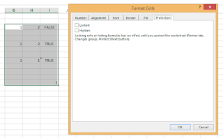
If you have any cells which you want the students to edit, such as a space to type their name, unlock these cells as well in the exact same way.
Hide the sensitive information
Next we'll hide the side cells. Highlight the columns with the secret information, then right click on the columns and click hide: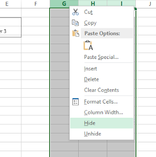
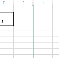
Password protect the sheet
Next we'll make it all password protected so that nothing can be changed except the option buttons. Go on Review - Protect Sheet - Set a password - OK: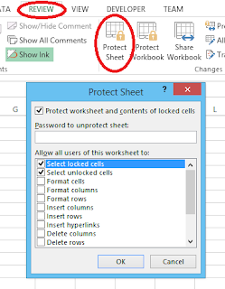
Also go on Review - Protect Workbook - Set a password - OK:
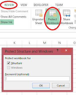
Now you have a multiple choice test sheet which cannot be tampered with.
STEP 8: Gathering the marks
The test has been taken and everyone saved their Excel sheet. Now you have to collect all the files and find everyone's mark. This would involve opening each file, unprotecting the sheet with your password, unhiding the hidden columns, and reading the mark at the bottom. Pretty daunting, but avoidable.You can use Excel to read the data in other Excel files. Just save a blank Excel file with all the answer files and add the following formula: "'[john smith.xlsx]Sheet1'!I13" where "john smith.xlsx" is the file name of the answer file, "Sheet1" is the Excel sheet name in the answer file, and "I13" is the cell containing the mark.

Just do this for all files and you've got a nice result sheet. If you want to give a correction you can even check the TRUE/FALSE column of each answer and say which questions were answered wrong. Use "IF('[john smith.xlsx]Sheet1'!I3, "Correct", "You said " & '[john smith.xlsx]Sheet1'!G3 & " instead of " & '[john smith.xlsx]Sheet1'!H3)" where I3 is the cell with the TRUE/FALSE result of the first question, G3 is the cell with the given answer, and H3 is the cell with the correct answer. You can even add another column in the answer sheet with a comment for whoever gets the question wrong.
Keep in mind that students might use a technique like this to read the hidden stuff in your answer file, but that shouldn't be easy to do without getting caught, especially if you hide a lot of columns (more than needed) and put the data in random columns.
The grid format
You can do your multiple choice in the below format where the sheet contains minimal information and the questions and candidate answers are on a printed sheet of paper.
This allows the students to scribble on the paper and to keep the Excel sheet short which saves scrolling.