Sunday, December 13, 2015

(k-)Nearest Neighbour(s) Classification

You want a computer to learn to assign objects into categories, such as the genre of a book. You happen to have a bunch of books with a known category. One of the simplest ways to make the computer assign an unknown book's category is to find the most similar book in the bunch to the unknown book and assume that the two books share the same category. For example, you want to find what genre "Harry Potter" is and find that it is most similar to a book you have called "The Hobbit" which is tagged as fantasy, so you conclude that "Happy Potter" is also fantasy. Of course this only makes sense if you have a big collection of reference books since there might not be any books which are similar otherwise, and the most similar book would be of a genre which is significantly different.

This is called the nearest neighbours classification algorithm, in particular the 1-nearest neighbour, because you only take into consideration the most similar book. Alternatively you can take the top 10 most similar books and use the most frequent genre among the 10 books. This would be called 10-nearest neighbours classification. In general it's called k-nearest neighbours classification.

This is a simple algorithm but its advantage is in its simplicity since it makes no assumptions about the data you give it. Whereas other machine learning algorithms assume that there is some simple pattern to decide which genre a book belongs to, the nearest neighbour classifier can discriminate between very complex patterns and will adapt to any data you train it with, provided that there is enough variety of data. The more complex the relationship between the books and the genre, the more variety of books you need to train it with.

The way it works is by first converting each book in your bunch into a bunch of lists of numbers called a vectors. Each vector would be a point in space (a vector of 2 numbers is a 2D point, of 3 numbers is a 3D point, and the rest are of high dimensional space). For example, in order to convert a book into a point, each number could be the number of times a particular word occurs. Create a vocabulary of words that matter, such as "wizard" and "gun", and then create a point consisting of the number of times each word occurs in the book. So if "Happy Potter" had "wizard" appearing 100 times and "gun" appearing 0 times, then it's 2D point would be (100, 0).

Next, compare the point version of the book in question to the point versions of every book in the bunch. Use some similarity measure to quantify how similar the points are. Similarity measures include Euclidean distance (normal distance between points) and Cosine similarity (difference in the angle of the points from the origin).


Which is the most similar point to the purple one in the above diagram (the purple point is (100, 0) which represents "Harry Potter")? The purple point will be of the same colour as the closest point.

Of course comparing to every point is slow, which is a problem given that nearest neighbour classification requires a lot of points to compare to. There are nearest neighbour search algorithms but they are not very efficient when the points have a lot of dimensions (many numbers in the vector). In some cases it is enough to use approximate search algorithms that do not give exact nearest point, but will find a reasonably close point quickly. The paper "Scaling Distributional Similarity to Large Corpora" gives an overview of such algorithms for finding words that have similar meanings.

If you do not have the genres of the books but still want to categorize similar books together you can use a clustering algorithm such as k-means clustering into order to group books by similarity and then use nearest neighbour classification to associate the new book with the group of the nearest book.

Friday, November 6, 2015

Naive Bayes Classification

The previous post was about Bayes' theorem, so now we'll talk about a use for it in machine learning: Naive Bayes Classification.

Let's say that you're making a program which given the content of a book, will tell you how likely it is that you will like it. In order to do so, it needs to know the contents of books that you like and books that you don't like. Parsing and understanding the content of a book is crazy hard, so you opt for a simpler strategy: You base the decision on the words used in the book. Books that you like use certain words that you like whilst books that you don't like use words that you don't like.

So you come up with a vocabulary of words (perhaps only a small set of words need to be considered) and you count the number of times each word appears a book you like and in a book you don't like. Let's say you end up with a table like this:

% of books that include word
Word\ClassLike bookHate book
magic100%0%
fairy90%10%
car5%95%
gun0%100%

This means that 90% of books that you like contain the word "fairy", which is another way of saying that a book with the word "fairy" has a 90% chance of being a good book.

Now we have a new book and we want to know if we're likely to like it or not. So we check which words it contains and find the following:
WordContained?
magicyes
fairyyes
carno
gunyes

The probability that you'll like the book given that it contains these words is found by calculating
P(Like book | magic=yes, fairy=yes, car=no, gun=yes)

Naive Bayes Classification works by first using Baye's theorem on the above conditional probability:
P(magic=yes, fairy=yes, car=no, gun=yes | Like book) P(Like book) / P(magic=yes, fairy=yes, car=no, gun=yes)

Now that the list of AND conditions (has magic and fairy and...) is at the front of the conditional, we can use the Naive Bayes Assumption and assume that the occurrence of each term is independent from all the other terms. If we assume this, we can simplify the probability by decomposing the ANDed conditions into separate probabilities multiplied together as follows:
P(magic=yes|Like book) P(fairy=yes|Like book) P(car=no|Like book) P(gun=yes|Like book) P(Like book) / (P(magic=yes) P(fairy=yes) P(car=no) P(gun=yes))

Now we can use the table at the top to find P(word|Like book), the probability P(Like book) is the percentage of books that you like (from those used to construct the table), and P(word) is the probability that a book contains the given word (from the books used to construct the table). These percentages are easy to obtain.

The problem is that one of our percentages is a zero, P(gun=yes | Like book). Because of this, when it is multiplied by the other probabilities, the result will be zero. The solution is to disallow zero probabilities by assuming that just because a word does not occur in the books you like, doesn't mean that it will never occur. It might be that there is a very tiny probability that it will occur, but that you don't have enough books to find it. In these situations, we need to smooth our probabilities using Laplace Smoothing by adding 1 to every count.

Naive Bayes Classification can be used to find the most likely class a list of yes/no answers belongs to (such as whether the book contains the given words), but this is just the simplest type of Naive Bayes Classification known as Bernoulli Naive Bayes, so called because it assumes a Bernoulli distribution in the probabilities (a Bernoulli distribution is when there are only 2 possible outcomes from an event with one outcome having a probability of "p" and the other "p-1"). It can also be used on a list of frequencies of the terms by using a Multinomial Naive Bayes or on a list of numbers with a decimal point (such as the weight of the book) using Gaussian Naive Bayes.

Saturday, October 3, 2015

Conditional probabilities and Bayes' theorem

So we all know that when a sports fan asks "What chance does our team have of winning?", the speaker is asking for a probability, but when that same person later asks "What chance does our team have of winning given that John will not be playing?", the speaker is now asking for a conditional probability. In short, a conditional probability is a probability that is changed due to the addition of new information. Let's see an example.

Conditional probabilities

Let's say that we have the following set of numbers, one of which is to be picked at random with equal probability:


The probability of each number being chosen is 1/7. But probabilities are usually based on subsets. So what is the probability of randomly choosing a square number from the above set?


The probability is, of course, 2/7. Now comes the interesting part. Let's say that the number is still chosen at random, but you have the extra information that the number that will be chosen is going to be an even number. In other words, although you don't know which number will be chosen, you do know that it will be an even number. What is the probability that the chosen number will be a square number?


Clearly the added information requires us to change the original probability of choosing a square number. We now have a smaller set of possible choices, only 2 (the red set). From these, there is only 1 square number (the intersection of the red and blue sets). So now the probability of choosing a square number is 1/2.

This is called a conditional probability. Whereas the first non-conditional probability is expressed as follows in mathematical notation:
P(number is square)
the second probability is a conditioned one and is expressed as follows:
P(number is square | number is even)
which is read as "probability that the number is square given that the number is even".

In general,
P(A|B) = P(A,B)/P(B)
where P(A|B) is the probability that event A occurs given that event B has occurred, P(A,B) is the probability that both events occur together (called the joint probability), and P(B) is the probability that event B occurred.


From this, we can derive some pretty interesting equations.

Bayes' theorem

First, it is clear from the above picture that it is straightforward to define P(B|A) by simply dividing by P(A):
P(B|A) = P(A,B)/P(A)

This means that:
P(B|A) P(A) = P(A,B)
and from the other formula, that:
P(A|B) P(B) = P(A,B)
which together mean that:
P(A|B) P(B) = P(B|A) P(A)
and
P(A|B) = P(B|A) P(A)/P(B)

This last equation is known as Bayes' theorem which is something that you'll encounter all the time in probability and artificial intelligence.

In many cases, the probability P(B) is difficult to find, but we can decompose it further by noticing that the probability of selecting from set B depends on whether or not a selection was made from set A. Specifically:
P(B) = P(A) P(B|A) + P(NOT A) P(B|NOT A)
This is saying that the probability of selecting from set B is equal to the probability of one of the following events occurring:
  • A selection is made from set A and it happens to also be an element in set B: P(A) P(B|A)
  • A selection is not made from set A but the selected element is in set B: P(NOT A) P(B|NOT A)

Thus Bayes' theorem can be rewritten as
P(A|B) = P(A) P(B|A) / ( P(A) P(B|A) + P(NOT A) P(B|NOT A) )

This is a more practical version of the formula. Let's see a practical example of it.

Bayes' theorem in action

Let's say that you have a robot that is trying to recognise objects in front of a camera. It needs to be able to recognise you when it sees you in order to greet you and fetch you your slippers. The robot sometimes makes mistakes. It sometimes thinks that it saw you when it did not (a false positive) and it sometimes sees you and doesn't realise it (a false negative). We need to calculate how accurate it is. Let's look at the following probability tree:


This tree is showing the following data:
P(you are there) = 0.1
P(you are not there) = 0.9
P(robot detects you | you are there) = 0.85
P(robot detects you | you are not there) = 0.15
P(robot does not detect you | you are there) = 0.05
P(robot does not detect you | you are not there) = 0.95

What is the probability that the robot detects you when you're there?
P(robot detects you AND you are there) =
P(robot detects you, you are there) =
P(you are there) P(robot detects you | you are there) =
0.1 x 0.85 = 0.085

Notice how we could have used the probability tree to calculate this (multiply the probabilities along a branch to AND them).

If the robot detects you, what is the probability that it is correct?
P(you are there | robot detects you) =
P(you are there) P(robot detects you | you are there) / ( P(you are there) P(robot detects you | you are there) + P(you are not there) P(robot detects you | you are not there) ) =
0.1 x 0.85 / ( 0.1 x 0.85 + 0.9 x 0.15 ) = 0.39

This is a small number, even though it correctly detects you 85% of the time. The reason is because you are in front of it only 10% of the time, which means that the majority of the time that it is trying to detect you you are not there. This will make that 15% of the time falsely detecting you pile up. One way to increase the accuracy is to limit the number of times an attempted detection is made in such a way that the probability that you are actually there is increased.

Bayesian inference

There is more to Bayes' theorem than using it to measure the accuracy of a robot's vision. It has interesting philosophical implications in epistemology. This is because it can be used to model the acquisition of knowledge. When used in this way we say that we are performing Bayesian inference. Let's say that you're a detective collecting clues on who committed a murder. You have a suspect in mind that you believe is the murderer with a certain probability. You find a clue which you believe is evidence that incriminates the suspect. This evidence should now increase your probability that the suspect is the murderer. But how do you find the new probability? Enter Bayes' theorem.

The probability you assigned to the suspect before the new evidence is P(H), the probability of the hypothesis, also known as the prior probability.
The new probability that you should assign to the suspect after discovering the evidence is P(H|E), also known as the posterior probability.
Now we use Bayesian inference to calculate the posterior probability as follows:

P(H|E) = P(H)P(E | H) / ( P(H)P(E | H) + P(NOT H)P(E | NOT H) )

The interpretation of this makes sense. The new probability given the evidence depends on two things:
  • The likelihood that the suspect was the murderer. The smaller this is, the stronger the evidence needs to be to make the hypothesis likely. This is described exactly by the quote "Extraordinary claims require extraordinary evidence".
  • The probability that the evidence would exist given that the suspect was not the murderer. It could be that the evidence actually supports the null-hypothesis, that is, that the suspect is actually not the murderer. This is determined by comparing the probability of the hypothesis with the probability of the null-hypothesis.

Finally notice also that if you have multiple hypothesis and want to see which is the most likely given a new evidence, we are essentially trying to find the maximum posterior probability of each hypothesis given the same evidence. Given the multiple competing hypothesis H_1, H_2, H_3, etc., the most likely H_i is found by:
argmax_i ( P(H_i)P(E | H_i) / ( P(H_i)P(E | H_i) + P(NOT H_i)P(E | NOT H_i) ) )
But we can simplify this by remembering that the denominator is P(E):
argmax_i ( P(H_i)P(E | H_i) / P(E) )
And of course since P(E) is a constant for each hypothesis, it will not affect which hypothesis will give the maximum posterior probability, so we can leave it out, giving:

argmax_i P(H_i)P(E | H_i)

Monday, September 14, 2015

How to make a multiple choice test using Excel

Here is a post for the teachers out there who are technologically savvy enough to use Excel but not quite enough to write a program or web application. It is easy to make your own multiple choice test in Excel which corrects itself, provided that it is feasible to make give a copy of the Excel file to each student and collect them all after the test. This also assumes that the risk of students not saving or accidentally deleting the file is negligible. But I know teachers who actually do this sort of thing so here is how to do it well.

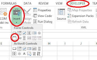
STEP 1: Activate "Developer" tab
Go on File - Options - Customize Ribbon - Select the "Developer" check box - OK:


STEP 2: Add a group box
Go on Developer - Insert - Group box in Form Control:


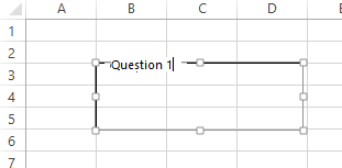
Then draw the group box and delete the text on it or write your question there:


STEP 3: Add option buttons
Go on Developer - Insert - Option button in Form Control:


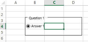
Then draw the option button COMPLETELY INSIDE the group box. This is very important, as if you don't draw it completely inside the group box, it will not be associated with other candidate answers of the same question and will not work properly. It's OK to move it outside of the group box afterwards but not before you draw it inside. Delete the text on the option button or write the candidate answer there:


STEP 4: Complete the test
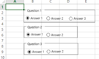
Repeat steps 3 and 2 as needed. If you need to reposition the form elements you first right click on them and then they are movable. Don't worry about accidentally selecting an option button; just make sure that checking an option button in a control group will not affect other control groups. If this happens then it is because the option buttons are not associated with the control group, because they were not drawn inside it, and you will have to draw a new one instead of it.


STEP 5: Automatically check the answers
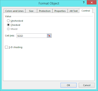
Right click on the option buttons - Format Control - Set Cell link to a particular cell:


You only need to set one of the option buttons for each question. Make sure that option buttons of different questions all use different cell links. While you're in the Format Control window you can unset any accidentally set option buttons.

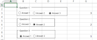
You now have the linked cell of each question contain a number which indicates the selected answer:


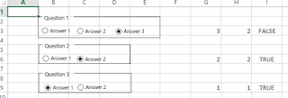
The number depends on the order in which the option buttons were added. Next write the correct answer next to each linked cell and next to that add a formula which checks if the right answer was selected. The formula is "=G3=H3" where "G3" is the linked cell and "H3" is the cell with the right answer.


The 3 columns on the side show the chosen answer (automatically set by the option buttons), the correct answer (entered by you), and whether the right answer was chosen or not (automatically set by a formula which compares the previous two).

STEP 6: Automatically compute the mark
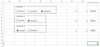
Finally, add the following formula under the TRUE/FALSE cells: "=COUNTIF(I3:I9,TRUE)" where "I3:I9" is the range of cells which are TRUE/FALSE.


STEP 7: Barricade the Excel sheet
At the moment the answers are in plain sight and everything is editable which makes it unsuitable for a test. So here's how to fix that.

Unlock the changing cells
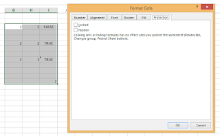
Start with setting the cells on the side to unlocked. This will allow the sheet to work when you lock it. Highlight the side cells (including the test mark), then right click - Format Cells - Protection - Uncheck both checkboxes:


If you have any cells which you want the students to edit, such as a space to type their name, unlock these cells as well in the exact same way.

Hide the sensitive information
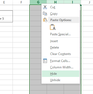
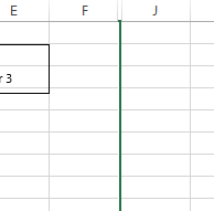
Next we'll hide the side cells. Highlight the columns with the secret information, then right click on the columns and click hide:


Password protect the sheet
Next we'll make it all password protected so that nothing can be changed except the option buttons. Go on Review - Protect Sheet - Set a password - OK:


Also go on Review - Protect Workbook - Set a password - OK:


Now you have a multiple choice test sheet which cannot be tampered with.

STEP 8: Gathering the marks
The test has been taken and everyone saved their Excel sheet. Now you have to collect all the files and find everyone's mark. This would involve opening each file, unprotecting the sheet with your password, unhiding the hidden columns, and reading the mark at the bottom. Pretty daunting, but avoidable.

You can use Excel to read the data in other Excel files. Just save a blank Excel file with all the answer files and add the following formula: "'[john smith.xlsx]Sheet1'!I13" where "john smith.xlsx" is the file name of the answer file, "Sheet1" is the Excel sheet name in the answer file, and "I13" is the cell containing the mark.


Just do this for all files and you've got a nice result sheet. If you want to give a correction you can even check the TRUE/FALSE column of each answer and say which questions were answered wrong. Use "IF('[john smith.xlsx]Sheet1'!I3, "Correct", "You said " & '[john smith.xlsx]Sheet1'!G3 & " instead of " & '[john smith.xlsx]Sheet1'!H3)" where I3 is the cell with the TRUE/FALSE result of the first question, G3 is the cell with the given answer, and H3 is the cell with the correct answer. You can even add another column in the answer sheet with a comment for whoever gets the question wrong.

Keep in mind that students might use a technique like this to read the hidden stuff in your answer file, but that shouldn't be easy to do without getting caught, especially if you hide a lot of columns (more than needed) and put the data in random columns.

The grid format
You can do your multiple choice in the below format where the sheet contains minimal information and the questions and candidate answers are on a printed sheet of paper.


This allows the students to scribble on the paper and to keep the Excel sheet short which saves scrolling.

Friday, August 7, 2015

Predicting the number of nodes in a trie with uniformly distributed strings

A trie is a type of tree that stores strings. Each character of the strings is a node and strings that share a common prefix also share the nodes, which means that a common prefix is only stored once, reducing some redundancy. But how much space is saved by using a trie? In order to answer this question, first we have to calculate the expected number of nodes a trie will have for "n" strings of "m" characters each with "c" possible characters (character set).

Consider the following diagram of a trie that contains the words "me", "if", "in", and "it". In it we have added a new word "my".


The word "my" only required the creation of one new node, since its first letter already existed in the word "me" so that node was shared and not recreated. In general, if a string is inserted in a trie, the number of new nodes created depends on the length of the longest existing prefix in the trie. This length will be the number of nodes that will be shared/reused. The remainder of the string will require new nodes for each character. If the whole string already exists then there will be 0 new nodes whilst if the string is completely new with no existing prefix then there will be a new node for each character. Specifically, for a string of length "m" whose longest existing prefix is of length "p", the number of new nodes created will be "m - p".

The equation we need to figure out looks like the following:
expected number of nodes = (m)(expected number of strings with prefix of length 1 not found)
                           + (m-1)(expected number of strings with prefix of length 2 not found)
                           + (m-2)(expected number of strings with prefix of length 3 not found)
                           + ...
                           + (1)(expected number of strings with prefix of length m not found)

Assuming that the strings are generated using a uniform distribution (any character can appear anywhere in the string), we need to find the expected number of strings out of "n" inserted strings made from "c" possible characters that will have a non-existing prefix of length "p".

This is basically the expected number of strings being selected for the first time when "n" selections are made from among all possible "p" length strings made from "c" possible characters (there are "c^p" possible such prefixes). This is equivalent to saying that it is the expected number of non-collisions when randomly placing "n" objects in "c^p" slots.

In my previous post, I showed that the expected number of collisions when randomly placing "n" objects in "s" slots is
n - s(1 - (1 - 1/s)^n)
which means that the number of non-collisions is
n - (n - s(1 - (1 - 1/s)^n))
which simplifies to
s(1 - (1 - 1/s)^n)
which when we plug in our values becomes
(c^p)(1 - (1 - 1/(c^p))^n)

But there's a problem. The above equation tells you the expected number of non-collisions when considering "p" length prefixes. But consider the previous diagram again. If the word "he" was added, it is true that the length 2 prefix of the word ("he") does not result in a collision, but this does not mean that just 1 new node will be added. In reality, 2 new nodes will be added because it is also true that its length 1 prefix ("h") will also not result in a collision. What this means is that the equation will not give the number of strings which will not result in a collision due to their length "p" prefix only, but also due to their length "p-1" prefix, which is not what we want. To fix this, we subtract from the equation the number of non-collisions due to the shorter prefix:
expected number of strings with prefix of length p not found = (c^p)(1 - (1 - 1/(c^p))^n) - (c^(p-1))(1 - (1 - 1/(c^(p-1)))^n)
Of course this does not apply for the length 1 prefix, so we need to be careful to only apply the subtraction for prefix lengths greater than one.
(You might think that we need to subtract for each shorter prefix length, but when this was tried the result became a negative number. Perhaps some form of inclusion-exclusion principle needs to be applied. Using this equation, the result matches empirical data for many different parameters.)

So, continuing from our earlier equation,
expected number of nodes = (m)((c^1)(1 - (1 - 1/(c^1))^n))
                           + (m-1)((c^2)(1 - (1 - 1/(c^2))^n) - (c^(2-1))(1 - (1 - 1/(c^(2-1)))^n))
                           + (m-2)((c^3)(1 - (1 - 1/(c^3))^n) - (c^(3-1))(1 - (1 - 1/(c^(3-1)))^n))
                           + ...
                           + (1)((c^m)(1 - (1 - 1/(c^m))^n) - (c^(m-1))(1 - (1 - 1/(c^(m-1)))^n))
= sum( c^i - c^i*((c^i-1)/c^i)^n for i in 1..m )

In Python code this becomes:
from fractions import Fraction
def exp_num_trie_nodes(n,m,c):
    return float(sum( c**i - c**i*Fraction(c**i-1,c**i)**n for i in range(1,m+1) ))

Rate of change

Here is a comparison of how the number of nodes increases depending of which variable (n,m,c) is changed:


As "n" increases, the number of nodes added starts slowing down, which makes sense since the more strings there are, the more existing prefixes can be reused. As "m" increases, the number of nodes added starts speeding up and then becomes linear, which makes sense too since longer strings are sparser and thus it would be harder to find a matching prefix which is long from among 100 strings. As "c" increases, the number of nodes added shoots up until a point where it then slows down, almost like it is logarithmic. This is because after a point it will not matter how rare the strings are since there are only 100 strings to choose from among the "c^m" possible strings. Since the length is not increasing, the same number of nodes will be used.

Size of trie

So does using a trie compress a set of strings? Keep in mind that a node takes more space than a character since it needs to point to other nodes whereas strings are arrays without pointers. We'll assume that all strings are the same length in order to reduce the number of variables. This will reduce the amount of information needed for both the set of strings and the trie (no need to include terminator flags for the strings) and the number of strings of maximum length is greater than the total number of shorter strings so it will not be a significant error in representation.

Call the number of nodes in the trie "N(n,m,c)".

The size of the normal set of strings is as follows:
n(m log(c))
where "log(c)" is the size of each character (the number of bits needed to represent each character). Of course this assumes that each string is unique. Tries only store unique strings and the way we compute the number of nodes does not assume that the strings will be unique. So we need to subtract the expected number of repeated strings from among those "n" strings. The number of repeated strings is equal to the number of collisions when placing "n" objects in "c^m" slots.
Array of strings: n(m log(c)) - (n - (c^m)(1 - (1 - 1/(c^m))^n))

The size of the trie is as follows:
N(n,m,c)(k(log(c) + log(N(n,m,c))))
where "log(c)" is the size of each character (the number of bits needed to represent each character), "log(N(n,m,c))" is the size of a pointer (which at minimum would be the logarithm of the number of nodes), and "k" is the number of pointers used on average per node. Given that the majority of the nodes in a trie will be leaf nodes, the majority of nodes will not have children. In fact the average will be less than one child per node. If arrays are used, "k" must be equal to "c", but if a linked list is used then "k" is the average but we have to also include the linked list pointer size with each character. The pointer size of the linked lists can be assumed to be "log(N(n,m,c))" since the total number of child nodes is equal to the number of nodes (minus the root node).
Array based: N(n,m,c)(c(log(c) + log(N(n,m,c))))
Linked list based: N(n,m,c)(k(log(c) + log(N(n,m,c)) + log(N(n,m,c))))

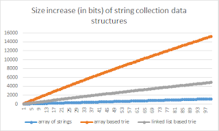
Here is a graph showing how the set of strings, array based trie, and linked list based trie increase in size with "n" when "c" is 5, "m" is 5, and "k" is 0.9:


It is clear that an array based trie cannot be used to compress a collection of strings as nodes take too much space. But what if we changed the value of "k" in the linked list based trie?


This shows that unless you have an average number of children per node of 0.2 or less, the array of strings will always take less space. Notice that this says nothing about tries which attempt to minimize the number of nodes such as radix trees where a single node represents a substring rather than a character. Also notice that this is about uniformly distributed strings, not linguistic strings which have a lot of redundancy. In a future post I shall make empirical comparisons on linguistic data.

Wednesday, July 8, 2015

Expected number of uniformly distributed collisions (birthday problem)

Here's an interesting mathematical problem. If you have "n" objects to be inserted into "m" available slots using a uniformly distributed random placement, how many collisions with already occupied slots should we expect to happen? This is useful for hashtables and other data structures where duplicates are not allowed.

Here is a Python 3 program that simulates inserting objects into random positions in an array and counting the average number of collisions.

def collisions(n, m):
 trials = 10000
 total_collisions = 0
 for _ in range(trials):
  slot_is_occupied = [ False for _ in range(m) ]
  for _ in range(n):
   slot = random.randint(0, m-1)
   if slot_is_occupied[slot]:
    total_collisions += 1
   else:
    slot_is_occupied[slot] = True
 return total_collisions/trials

Here is a sample of the average number of collisions given by the above function for different values of "n" and "m":
n\m12345678910
10.00.00.00.00.00.00.00.00.00.0
21.00.49470.33340.25150.20540.1630.14370.12970.11180.1053
32.01.24470.88610.6850.5570.46330.40230.35370.3250.2819
43.02.12911.58121.25881.04430.90540.77540.69240.61760.5459
54.03.06172.41.9441.64571.42041.23641.11230.99840.9019
65.04.0343.2652.70782.3042.02181.76041.60041.43491.318
76.05.01684.17423.54063.04982.67162.39732.14991.94171.7744
87.06.00755.12064.4033.83633.39053.03042.73782.51512.3219
98.07.00356.07655.30524.67884.16523.7383.41683.12052.8816
109.08.00167.05266.22335.54014.96324.4934.09133.77213.5016

Basically the answer is the number of objects "n" minus the number of occupied slots. This will give us the number of objects excluding the ones which were inserted without collision, that is, in an empty slot. For example, if I insert 5 objects into an array but at the end there are only 3 occupied slots, then that must mean that 2 of those objects were inserted in the same slot as some other objects (they collided with them).

The question is how to predict the expected number of occupied slots.

Expected number of occupied slots

What is the average number of slots ending up being occupied by at least one object? This previous blog post explains that you basically just need to multiply the probability of a given slot being occupied at the end by the number of slots. So what is the probability of a slot being occupied?

Probability of a slot being occupied

What is the probability that an object is inserted into a particular slot out of "m" slots?
1/m

Therefore the probability that the slot remains empty is
1 - 1/m

What is the probability that the slot is still empty after another placement? It's the probability that the first object did not land on the slot AND that the second object did not land on the slot too. These two probabilities are independent of each other, so
(1 - 1/m)(1 - 1/m)

In general, after "n" objects have been placed, the probability that the slot is still empty is
(1 - 1/m)^n

Notice that this makes sense for n = 0 because if no objects were placed, then the probability that the slot is empty is 1.

Which means that after "n" objects have been placed, the probability that the slot is occupied is
1 - (1 - 1/m)^n

Therefore...

Therefore, the expect number of occupied slots among "m" slots after "n" objects have been inserted with uniform probability is
m(1 - (1 - 1/m)^n)

Which means that the expected number of collisions is
n - m(1 - (1 - 1/m)^n)

Here is the same table as the one at the top showing the corresponding predicted number of collisions:

n\m12345678910
10.00.00.00.00.00.00.00.0-0.00.0
21.00.50.33330.250.20.16670.14290.1250.11110.1
32.01.250.88890.68750.560.47220.40820.35940.3210.29
43.02.1251.59261.26561.0480.89350.77840.68950.61870.561
54.03.06252.39511.94921.63841.41131.23871.10330.99440.9049
65.04.03133.26342.71192.31072.00941.7761.59041.43941.3144
76.05.01564.17563.53393.04862.67452.37942.14161.94621.783
87.06.00785.11714.40053.83893.39543.03952.74892.50772.3047
98.07.00396.0785.30034.67114.16283.74813.40533.1182.8742
109.08.0027.0526.22535.53694.9694.49844.10463.77153.4868

The maximum absolute error between the two tables is 0.0179.

Probabilities are average proportions (expected value)

Intuitively, if a coin flip has a probability of 1/2 of turning out heads, and we flipped the coin 100 times, we expect that 1/2 of those 100 flips will be heads. What is meant by "expect" is that if we do this 100 coin flip experiment for many times, count the number of times it turns out heads for each 100 flip trial, and take the average of these counts, the average will be close to 1/2 of 100. Furthermore, the more 100 flip trials we include in our average, the closer the average will be 1/2 of 100.

If this were the case, then a probability can be treated as an average proportion, because if a probability of something happening is, say, 1/100, then after 1000 attempts we should find that, on average, 1/100 of those 1000 attempts would be the thing happening. In general, if the probability of an outcome is "p", and "n" attempts are made, then we should have "pn" positive outcomes. That probability is acting as a proportion of the average number of attempts made which will result in a positive outcome out of the attempts made. In fact, semantically speaking, the phrase "This outcome occurs with probability 1/100" and the phrase "This outcome occurs once every 100 times" are identical.

A simple proof of this is in the way we estimate the probability of an outcome. We attempt to produce the outcome (such as a coin flip resulting in heads) for a number of times "n", count the number of times "x" the outcome is positive (heads), and then just find x/n. But in order for this probability to be reliable, the quotient must remain constant for different values of "n" (the value "x" will change according to "n" to keep x/n equal). Given this statement, if we know a reliable probability x/n, and have performed the experiment "m" times, then the number of positive outcomes "y" can be predicted as follows:
For x/n to be reliable, x/n = y/m
Therefore, y = m(y/m) = m(x/n)
That is, since x/n is known and "m" is known, "y" can be found using those two values only.

Of course this is not a rigorous proof. To get a rigorous proof we need to turn to a field of probability called expected value. The expected value of a random variable (such as a coin flip) is the average of the values (assumed to be numerical) of the outcomes after a large number of trials. It is defined as the sum of each outcome multiplied by its probability. For example, the expected value of the value on a die is
1*1/6 + 2*1/6 + 3*1/6 + 4*1/6 + 5*1/6 + 6*1/6
because for each outcome from 1 to 6, the probability is 1/6.

In general, if the probability of outcome "o_i" is "p_i", then the expected outcome is
sum(o_i*p_i for all i)

But this isn't useful for proving the statement in the title. The proof is in this Math Exchange answer which explains that the expected number of positive outcomes out of "n" attempts, given that the probability of each outcome each time is "p", is "pn". It goes like this:

Let the random variable "U_i" be the outcome of the "i"th attempt (heads or tails). If the outcome is positive (heads), "U_i" is 1, otherwise it is 0. Given "n" attempts, the number of positive outcomes is
U_1 + U_2 + U_3 + ... + U_n

Call this actual number of positive outcomes "X", that is
X = U_1 + U_2 + U_3 + ... + U_n

The expected value of "X", written as E(X) is
E(X) = E(U_1 + U_2 + U_3 + ... + U_n)

Since the expected value is a linear operator,
E(X) = E(U_1) + E(U_2) + E(U_3) + ... + E(U_n)

Now, given the above definition of what an expected value is,
E(U_i) = 1*(probability of U_i = 1) + 0*(probability of U_i = 0)

If the probability of "U_i" being 1 is "p_i", then
E(U_i) = p_i

But for all "i", the probability of "U_i" is the same. That is
E(U_i) = p

So that means that
E(X) = p + p + p + ... + p
E(X) = pn

And there we have it, the expected number of positive outcomes out of "n" attempts, each of which has a probability of "p", is "pn", which means that the probability "p" can be treated exactly as if it was the proportion of positive outcomes out of a number of trials.

Wednesday, June 24, 2015

Compressed frequencies: Representing frequencies with less bits

In a cache memory you usually store the most frequently used data that is currently in a larger but slower memory. For example, you keep your most frequently accessed files cached in RAM rather than on your hard drive. Since you can't fit all the contents of your hard disk in RAM, you keep only the most frequently used files that can fit. You will still need to access your hard disk once in a while in order to access your less frequently used files but the average file access time will now be greatly reduced.

The problem is how to keep count of the number of times each file is being used in order to know which is the most frequently used. The obvious solution is to associate each file with a number and increment that number each time it is used. But numbers take space as well, and sometimes this becomes a significant problem. You might not afford to waste 4 or 8 bytes of memory worth of frequency integers for every item. Is there a way to bring down the number of bytes used by the frequency integers without losing their usefulness?

Here is an example of a 4 byte int integer number in memory representing the number 45723:
00000000 00000000 10110010 10011011

The most obvious thing you can do is to tear away the most significant bits (the ones on the left which have a larger value) by using smaller range number types such as the 2 byte short, which gives us 10110010 10011011. If the frequency is sometimes, but rarely, larger than the ranges provided by these smaller types, then you can just cap it off by stopping incrementation once the maximum number is reached. For example, if we're using a two byte short, then the maximum number this can be is 65535. Once the frequency reaches this number, then it gets frozen and never incremented again. Many frequences follow a zipfian distribution, meaning that the vast majority of items will have a small frequency, followed by a handful of very frequent items. An example of this is words in a document where most words will only occur once and only a few words such as "the" and "of" will occur frequently. If this is the case then you will be fine with capping off your frequencies since only a few items will have a large frequency and it might not be important to order these high frequency items among themselves.

It might seem more useful instead to tear away the least significant bits (the ones on the right which have a smaller value) instead, since these are less useful. The way you do this is to divide the frequency by a constant and keep only the whole number part. For example, if we divide the above number by 256, we'd be shifting the bits by one byte to the right, which gives us 00000000 00000000 00000000 10110010. The least significant byte has been removed which means that we can use less bytes to store the frequency. But in order to do that you need to first have the actual frequency which defeats the purpose. So what we can do is to simulate the division by incrementing the frequency only once every 256 times. If we do that then the resulting number will always be a 256th of the actual frequency which is the frequency without the least significant byte. But how do you know when to increment the frequency next? If you keep a separate counter which counts to 256 in order to know when to increment next then you lose the space you would have saved. Instead we can do it stochastically using random numbers. Increment the frequency with a probability of 1 in 256 and the frequency will be approximately a 256th of the actual frequency.

By combining these two ideas together we can reduce an 8 byte frequency into a single byte and that byte will be one of the original 8 bytes of the actual frequency. Here is a Python function that increments an integer with a compressed frequency that is a certain number of bytes long and with a certain number of least significant bytes torn off.

def compressed_increment(frequency, bytes_length, bytes_torn):
    if frequency < 256**bytes_length: #cap the frequency to the maximum number that can be contained in bytes_length bytes
        if random.randint(1, 256**bytes_torn) == 1: #increment with a probability of 1 in 256^bytes_length (number to divide by to shift the frequency by that number of bytes)
            return frequency + 1

Of course this is a lossy compression. Information is lost. This means that the compressed frequency is not useful in certain situations, such as when you want to also decrement the frequency or when approximate frequencies are inadequate.

Saturday, May 23, 2015

Translating an arbitrary integer into a circular array index

A circular array is an array which is connected at the edges, that is, it has no beginning or end and traversing the array will eventually get you back to where you started. Of course in practice a normal array is used and the given index is mapped into a valid array index. This is usually done using modulo operations (the remainder after dividing the index by the array length). But what if you need to also allow negative indexes?

Let's say you have an array of length 5 and you want to use it as a circular array.

01234

If you start at index 2 and move 1 to the right then you end up in index 3. But if you move 3 to the right you end up in index 0. On the other hand if you move 3 to the left then you end up in index 4. Here are some other examples of this translation:

Starting indexAdd to itResultantTranslated index
2+133
2-122
4+150
0-1-14
2+340
2-3-14
2+794
2-7-50
2+15172
2-15-132

We need a general formula to map arbitrary resultant integers into corresponding indexes. The modulo operator will not map negative numbers correctly:

6 % 5 = 1
5 % 5 = 0
4 % 5 = 4
3 % 5 = 3
2 % 5 = 2
1 % 5 = 1
0 % 5 = 0
-1 % 5 = -1
-2 % 5 = -2
-3 % 5 = -3
-4 % 5 = -4
-5 % 5 = 0
-6 % 5 = -1

This is because if the whole number division of a negative number N divided by a positive number P is D, then the remainder would be the number X such that D*P + X = N holds. For example, 4/5 = 0 remainder 4, because 0*5 + 4 = 4. Another example, -4/5 = 0 remainder -4 because 0*5 + -4 = -4.

Now in order to get a mapping from arbitrary resultant integers to corresponding indexes in a circular array we need to use the following formula:

Given a resultant R and a length of array L, the corresponding index is
(R%L + L)%L

Wednesday, March 25, 2015

Fractions and decimals

Let's take a break from irrational numbers and focus a bit on the rational ones. Rational numbers can be either be of a fixed number of decimal digits such as 0.123, called terminating decimals, or have a part of its decimal digits which repeat forever such as 0.272727..., called recurring decimals. Both terminating and recurring decimals can be represented as fractions. Let's see how to convert one to the other.

Fraction to decimal

Terminating decimals

The way to convert a fraction to a decimal is of course through the familiar long division algorithm, which was already shown in a previous blog post of mine. The way I show it here is how I learned it at school, which is a fast method but which leaves nearly nothing explained in its working. Let's convert 43/5 to decimal form:

          
5 )4 3

We start by seeing how many times the denominator 5 goes into the first digit of the numerator, 4. It goes 0 times into it and leaves a remainder of 4. We write the integer quotient as the first digit at the top. The remainder we write in front of the next digit in the numerator.

   0         
5 )4 43

We now see how many times 5 goes into 43. It goes 8 times into it and leaves 3 as a remainder. We write the integer quotient as the second digit at the top. We now have no more digits in the numerators, so we add a decimal point and a zero after it to create more digits. We also add a decimal point to the quotient at the top.

   0  8 .     
5 )4 43 . 30

And repeat.

   0  8 .  6  
5 )4 43 . 30 00

Since the last remainder was 0, if we had to continue from here onwards we'd be adding nothing by zeros to the top quotient which would be pointless. So instead we declare the number as terminating decimal and stop there. The answer the top quotient, that is, 43/5 = 8.6

What's happening here is that we're first trying to find the tens digit of the quotient by seeing how many times 50 goes into 43 which is 0 (tens) remainder 43. Then we're trying to find the units digit of the quotient by seeing how many times 5 goes into 43 which is 8 (units) remainder 3. Then we're trying to find the tenths digit of the quotient by seeing how many times 0.5 goes into 3, or equivalently, how many times 5 goes into 30, which is 6 (tenths) remainder 0.

Recurring decimals

Let's use the previous method to convert 1/3 to decimal form:

          
3 )1

We start by seeing how many times the denominator 3 goes into the first digit of the numerator, 1. It goes 0 times into it and leaves a remainder of 1.

   0 .       
3 )1 . 10

We now see how many times 3 goes into 10. It goes 3 times into it and leaves 1 as a remainder.

   0 .  3    
3 )1 . 10 10

And repeat.

   0 .  3  3 
3 )1 . 10 10 10

As you can see, this process will continue indefinitely, meaning that the 3 at the top will keep on repeating itself. This makes the quotient a recurring decimal, the proof of which is that one of the remainders after the decimal point was reached appeared twice and hence the same number must come out again.

Decimal to fraction

Terminating decimals

To convert a terminating decimal to a fraction you simply multiply it by a power of 10 that is large enough to make it a whole number, then put that same power of 10 as the denominator under the whole number. For example, if you have 12.3456 to convert to fraction form:

12.3456 = 12.3456 x 10000 / 10000
        = 123456/10000
        = 7716/625

Recurring decimals

Of course the previous method cannot be used when the fractional part is infinitely long. But there is a trick we can use. The fraction 1/9 has the following decimal expansion:

   0 .  1  1 ...
9 )1 . 10 10 ...

In other words, it gives a decimal number with an infinite sequence of 1s. We can use this to our advantage so that we can obtain infinite sequences of any digit by simply multiplying the digit by 1/9.

1/9 = 0.111...
2/9 = 0.222...
3/9 = 0.333...
etc

The interesting thing about this is that when you try to get an infinite sequence of 9s, you get the whole number 1. This is one of the proofs that 0.999... = 1.

But this is only good for single digit recurrences. For two digit recurrences we can use 1/99:

    0 .  0  1  0  1 ...
99 )1 . 10 100 10 100 ...

This is useful. We can replace every 1 with any digit by multiplying 1/99 by that digit.

1/99 = 0.0101...
2/99 = 0.0202...
3/99 = 0.0303...
etc

We can also shift those digits one place to the left by multiplying the digit by 10:

10/99 = 0.1010...
20/99 = 0.2020...
30/99 = 0.3030...
etc

So we can control both digits by adding these two fractions together:

10/99 + 3/99 = 0.1010... + 0.0303... = 0.1313...

Which of course simplifies to

13/99 = 0.1313...

That is, you just multiply the 2 digit number you want to be repeated by 99.

Can this be extended to any number of digits? 1/999 gives the following expansion:

     0 .  0  0   1  0  0   1 ...
999 )1 . 10 100 1000 10 100 1000 ...

So with 1/999 we can repeat any 3 digit recurrences. With each new 9 added to the denominator we are postponing the number of times the remainder must be moved before it is big enough to be divided by the denominator. That postponement results in another 0 added to the recurring decimal.

So in short, to convert a recurring decimal number to a fraction, just take the repeating part of the decimal and put it over a denominator consisting of as many 9s as there are digits in the repeated number:

0.01230123... = 0123/9999

But this will only work if the decimal number consists of nothing but repeating numbers. What if you have the following decimal:

210.67801230123...

In this case, the repeating part is the "0123" but it starts with other non-repeating digits. Not to worry, we just separate the two parts of the number into a sum:

210.67801230123... = 210.678 + 0.00001230123...

The recurring term can be multiplied by a power of 10 that will make it lose its leading zeros. Of course we can't just multiply it by a power of 10 without also dividing it by the same number in order to avoid changing its value:

210.67801230123... = 210.678 + (1000 x 0.00001230123... / 1000)
210.67801230123... = 210.678 + (0.01230123... / 1000)

We can now convert each term separately:

210.67801230123... = 210.678 + (0.01230123... / 1000)
                   = 210678/1000 + ((0123/9999) / 1000)
                   = 140437963/666600

Saturday, February 7, 2015

Finding the nth row in every group in SQL

Let's say you have the following log table which stores the dates of each access:

TimeStampIPUserName
2005-10-30 10:45:03172.16.254.10jlor
2005-10-30 10:46:31172.16.254.12kpar
2005-10-31 09:14:13172.16.254.14jlor
2005-10-31 09:25:42172.16.254.16kpar
2005-10-31 12:41:14172.16.254.19jlor
2005-11-01 07:15:15172.16.254.20kpar

You are asked to make a report of the last time each user has accessed the system using SQL.

At first you try using GROUP BY but then realize that it's not so simple to include the IP field along with the TimeStamp and UserName. GROUP BY works when you're interested in aggregating every field that is not used to group the records. In other words, you can easily do this:

SELECT UserName, MAX(TimeStamp)
FROM log
GROUP BY UserName

USERNAMEMAX(TIMESTAMP)
jlorOctober, 31 2005 12:41:14+0000
kparNovember, 01 2005 07:15:15+0000

But if you also want to show the corresponding IP address of the access with the latest time stamp, you'd have a problem using simple SQL. If you add the IP field in the SELECT statement, you'd end up with the first IP in the table that belongs to the corresponding user, rather than the IP of the latest time stamp.

SELECT UserName, IP, MAX(TimeStamp)
FROM log
GROUP BY UserName

USERNAMEIPMAX(TIMESTAMP)
jlor172.16.254.10October, 31 2005 12:41:14+0000
kpar172.16.254.12November, 01 2005 07:15:15+0000

The way to do this is to simulate the GROUP BY statement using more expressiveness methods.

MS SQL Server

In MS SQL Server, this is achieved using the ROW_NUMBER function. This function gives a number for each row (1, 2, 3, ...) which can be used inside a SELECT statement. The cool thing about this function is that the numbering can be made to restart for every different value in a field. So if we used it on the UserName field we'd have the following:

SELECT UserName, IP, TimeStamp, ROW_NUMBER() OVER(PARTITION BY UserName ORDER BY TimeStamp DESC)
FROM log

USERNAMEIPTIMESTAMPCOLUMN_3
jlor172.16.254.10October, 30 2005 10:45:03+00001
jlor172.16.254.14October, 31 2005 09:14:13+00002
jlor172.16.254.19October, 31 2005 12:41:14+00003
kpar172.16.254.12October, 30 2005 10:46:31+00001
kpar172.16.254.16October, 31 2005 09:25:42+00002
kpar172.16.254.20November, 01 2005 07:15:15+00003

It even orders the rows by user name and it lets you say how you want the rows of each user to be ordered so that you can say how you want the numbering. Using the SQL above, the row with the latest time stamp of each user has a 1 in the last column. This allows us to select it. It will have to be inside a nested query however in order to be used in a WHERE statement.

SELECT UserName, IP, TimeStamp
FROM (
  SELECT UserName, IP, TimeStamp, ROW_NUMBER() OVER(PARTITION BY UserName ORDER BY TimeStamp DESC) AS rank
  FROM log
) AS t
WHERE rank = 1

USERNAMEIPTIMESTAMPCOLUMN_3
jlor172.16.254.19October, 31 2005 12:41:14+0000
kpar172.16.254.20November, 01 2005 07:15:15+0000

Notice that you can even find when the second to last time an access was made by changing the 1 in the WHERE statement to a 2.

You can experiment with this in this SQL Fiddle.

MySQL
Unfortunately MySQL doesn't have a function as nifty as ROW_NUMBER so instead we'll have to simulate that using variables. In MySQL you can create variables using the SET statement and then update them within a SELECT statement so that they change for each row, like this:

SET @row_number := 0;
SELECT UserName, IP, TimeStamp, @row_number := @row_number + 1
FROM log

USERNAMEIPTIMESTAMP@ROW_NUMBER := @ROW_NUMBER + 1
jlor172.16.254.10October, 30 2005 10:45:03+00001
kpar172.16.254.12October, 30 2005 10:46:31+00002
jlor172.16.254.14October, 31 2005 09:14:13+00003
kpar172.16.254.16October, 31 2005 09:25:42+00004
jlor172.16.254.19October, 31 2005 12:41:14+00005
kpar172.16.254.20November, 01 2005 07:15:15+00006

This is only half the story of course. We want the numbering to restart for every user and we also want this to happen after sorting the rows by user name. We also want the rows belonging to each user to be sorted by time stamp. A simple ORDER BY statement can handle the sorting part:

SET @row_number := 0;
SELECT UserName, IP, TimeStamp, @row_number := @row_number + 1
FROM log
ORDER BY UserName, TimeStamp DESC

USERNAMEIPTIMESTAMP@ROW_NUMBER := @ROW_NUMBER + 1
jlor172.16.254.19October, 31 2005 12:41:14+00001
jlor172.16.254.14October, 31 2005 09:14:13+00002
jlor172.16.254.10October, 30 2005 10:45:03+00003
kpar172.16.254.20November, 01 2005 07:15:15+00004
kpar172.16.254.16October, 31 2005 09:25:42+00005
kpar172.16.254.12October, 30 2005 10:46:31+00006

The restarting of numbering is a little less simple. We have to keep track of what the previous value was using another variable and we have to also choose between setting row_number to 1 or to increment it by 1. Here is the code:

SET @row_number := 0;
SET @prev_username := NULL;
SELECT UserName, IP, TimeStamp, @row_number := CASE WHEN UserName = @prev_username THEN @row_number + 1 ELSE 1 END, @prev_username := UserName
FROM log
ORDER BY UserName, TimeStamp DESC

USERNAMEIPTIMESTAMP@ROW_NUMBER := CASE WHEN USERNAME = @PREV_USERNAME THEN @ROW_NUMBER + 1 ELSE 1 END@PREV_USERNAME := USERNAME
jlor172.16.254.19October, 31 2005 12:41:14+00001jlor
jlor172.16.254.14October, 31 2005 09:14:13+00002jlor
jlor172.16.254.10October, 30 2005 10:45:03+00003jlor
kpar172.16.254.20November, 01 2005 07:15:15+00001kpar
kpar172.16.254.16October, 31 2005 09:25:42+00002kpar
kpar172.16.254.12October, 30 2005 10:46:31+00003kpar

The CASE statement selects a value to set row_number. If the current row's user name is the same as the previous one's then the value will be one more than row_number it currently is. Otherwise it is set to 1. After that variable is set, the prev_username variable is set to the current row's user name.

Finally we can now use this to select the latest access for each user.

SET @row_number := 0;
SET @prev_username := NULL;
SELECT UserName, IP, TimeStamp
FROM (
  SELECT UserName, IP, TimeStamp, @row_number := CASE WHEN UserName = @prev_username THEN @row_number + 1 ELSE 1 END AS rank, @prev_username := UserName
  FROM log
  ORDER BY UserName, TimeStamp DESC
) AS t
WHERE rank = 1

USERNAMEIPTIMESTAMP
jlor172.16.254.19October, 31 2005 12:41:14+0000
kpar172.16.254.20November, 01 2005 07:15:15+0000

Notice that you can even find when the second to last time an access was made by changing the 1 in the WHERE statement to a 2.

You can experiment with this in this SQL Fiddle.

Saturday, January 31, 2015

The Lempel Ziv Welch (LZW) compression algorithm

The Lempel Ziv Welch algorithm (LZW) is a classic compression algorithm published in 1984. It's a simple but practical algorithm that should be under every geek's belt and is often used in combination with other techniques.

The basic idea
Let's start with a plain English description of how this algorithm works. Let's say that we want to compress the following input string:

xxxxyyyyxxxxxxxxxxxx


Compression

If we're lazy, all we have to do to produce a valid output is to represent each letter using 2 characters.

0x0x0x0x0y0y0y0y0x0x0x0x0x0x0x0x0x0x0x0x

According to the compressed language of LZW, when a character pair starts with a "0", that means that the second character is the original letter. This has doubled the size of the sequence, but hopefully this is not the actual output. When the first character is something other than "0", the character pair becomes a reference to some prior long sequence. These references are what will compress the sequence.


In order to compress, we need to use a special table called a "dictionary" which maps 2 character values to the string they represent. Right off the bat, the dictionary will start with the following values:

Actual string2 character value
a0a
b0b
......
x0x
y0y
z0z

We start scanning through the input string from the first letter and find the longest sequence of letters which are in the dictionary. At this point, that would obviously be the first letter, since the dictionary only have single letters.

xxxxyyyyxxxxxxxxxxxx

After finding the longest string from the start which is in the dictionary, "x", including also the next letter in the input will make the shortest string which is not in the dictionary. This unregistered string is "xx".

We replace the longest string found in the dictionary with the corresponding 2 character value:

0xxxxyyyyxxxxxxxxxxxx

The next shortest string not in the dictionary is then added to the dictionary.

Actual string2 character value
a0a
b0b
......
z0z
xx1a

Now we continue scanning the input string from after the last replacement.


Again, we look for the longest string that is in the dictionary. That would be "xx", which we added in the previous step.

0xxxxyyyyxxxxxxxxxxxx

We replace this string with the corresponding 2 character value and add into the dictionary this string plus the next letter ("xxx").

0x1axyyyyxxxxxxxxxxxx

Actual string2 character value
a0a
......
z0z
xx1a
xxx1b

Repeat the process from right after the last replacement.


0x1axyyyyxxxxxxxxxxxx

This time it was "x" on its own that was the longest string in the dictionary since "xy" was not in the dictionary.

0x1a0xyyyyxxxxxxxxxxxx

Actual string2 character value
......
z0z
xx1a
xxx1b
xy1c

Repeat.


0x1a0xyyyyxxxxxxxxxxxx

Longest string in dictionary was "y", shortest string not in dictionary was "yy".

0x1a0x0yyyyxxxxxxxxxxxx

Actual string2 character value
......
z0z
xx1a
xxx1b
xy1c
yy1d

Repeat.


0x1a0x0yyyyxxxxxxxxxxxx

Longest string in dictionary was "yy", shortest string not in dictionary was "yyy".

0x1a0x0y1dyxxxxxxxxxxxx

Actual string2 character value
......
z0z
xx1a
xxx1b
xy1c
yy1d
yyy1e

Repeat.


0x1a0x0y1dyxxxxxxxxxxxx

Longest string in dictionary was "y", shortest string not in dictionary was "yx".

0x1a0x0y1d0yxxxxxxxxxxxx

Actual string2 character value
......
xx1a
xxx1b
xy1c
yy1d
yyy1e
yx1e

Repeat.


0x1a0x0y1d0yxxxxxxxxxxxx

Longest string in dictionary was "xxx", shortest string not in dictionary was "xxxx".

0x1a0x0y1d0y1bxxxxxxxxx

Actual string2 character value
......
xx1a
xxx1b
xy1c
yy1d
yyy1e
yx1e
xxxx1f

Repeat.


0x1a0x0y1d0y1bxxxxxxxxx

Longest string in dictionary was "xxxx", shortest string not in dictionary was "xxxxx".

0x1a0x0y1d0y1b1fxxxxx

Actual string2 character value
......
xx1a
xxx1b
xy1c
yy1d
yyy1e
yx1e
xxxx1f
xxxxx1g

Repeat.


0x1a0x0y1d0y1b1fxxxxx

Longest string in dictionary was "xxxxx" which resulted in the whole input string being consumed, hence there is nothing left to add to the dictionary.

0x1a0x0y1d0y1b1f1g


0x1a0x0y1d0y1b1f1g

This has resulted in an output string which is 2 characters shorter. Obviously the string was engineered to be compressed. Had it been a longer string then the dictionary would have contained longer strings which would lead to more compression.


Decompression
Compression is quite straightforward and so should decompression. Except that it's a little less straightforward because of a special case that can sneak up on you if you don't know about it (some online sources don't mention it).

If we knew what the dictionary contains then we can simply replace each 2 character value with its corresponding string. But in order to know from the start what the dictionary is we would have to include it with the output string, which would be a considerable amount of extra bytes. Instead, decompression basically consists of guessing what the dictionary contained one 2 character value at a time.


We start with the obvious. The dictionary surely contained all the single letters.

Actual string2 character value
0aa
0bb
......
0xx
0yy
0zz

The 2 character value is always one of the above initial dictionary (since that is the first shortest string not in the dictionary), so we go ahead and take care of that.

0x1a0x0y1d0y1b1f1g

x1a0x0y1d0y1b1f1g

From here on, if a 2 character value is in the dictionary then we just replace it with its corresponding string. After each replacement we use the replaced string to update the dictionary (as will be shown in an examples further down). The problem is if the 2 character value is not in the dictionary, as is the case now. This is the special case.


The next 2 character value is not in the dictionary. But notice that it is the very next 2 character value that will enter the dictionary, "1a". When this is the case, the following scenario must have taken place:

The input string has been determined to start with an "x", but the following letters are unknown.
x _ _ _

We know that the following letters were replaced with the next available 2 character value (from the compressed string), which means that it must be the shortest string that was not in the dictionary after "x" was replaced with "0x".

This shortest string must have been the last string that was replaced with a 2 character value ("x"), plus the letter after it. So the dictionary must have looked something like this:

Actual string2 character value
......
0xx
0yy
0zz
1ax_

(Notice that the blank is an unknown letter)

So then the first letter of this unknown string being referred to by the 2 character value "1a" is "x". In that case then we know what the second letter is in the input string: an "x", according to the dictionary we're constructing.

x x _ _

But wait, since the 2 character value "1a" is referring to the first "x" followed by the next letter, and since we have determined that the next letter was "x", then "1a" must be referring to "xx".

Actual string2 character value
......
0xx
0yy
0zz
1axx

In general, every time we encounter this situation, where 2 character value is not in the dictionary and is the next value to be added to the dictionary, the string being referred to is the previous replaced string followed by the same string's first letter. In this case, the previous replaced string was "x" whose first letter is "x", so the string referred to by "1a" is "xx".

x1a0x0y1d0y1b1f1g

xxx0x0y1d0y1b1f1g

After every replacement after the very first (this is the second), we need to update the dictionary with a new 2 character value. The update needs to reflect what was added during compression when the previous replacement (the first in this case) took place. This is because you need to know what letter follows the replacement in order to know which string was added to the dictionary.

Remember that during compression we were adding to the dictionary the shortest string that was not in the dictionary, which consisted of the longest string found in the dictionary (the replaced string) followed by the next letter. After the very first replacement we made, the "x", the next letter in the string is the first letter of the second replacement we made, the "xx". So we add to the dictionary the previous replacement followed by the first letter of the current replacement.

Actual string2 character value
......
0xx
0yy
0zz
1axx

Finally we've covered all the steps needed to get repeatin'. Let's continue.


xxx0x0y1d0y1b1f1g

This one is easy as it is already in the dictionary.

xxxx0y1d0y1b1f1g

The previous replacement was "xx", the current replacement was "x". So to the dictionary we add "xxx".

Actual string2 character value
......
0xx
0yy
0zz
1axx
1bxxx

Repeat.


xxxx0y1d0y1b1f1g

In the dictionary.

xxxxy1d0y1b1f1g

The previous replacement was "x", the current replacement was "y". So to the dictionary we add "xy".

Actual string2 character value
......
0xx
0yy
0zz
1axx
1bxxx
1cxy

Repeat.


xxxxy1d0y1b1f1g

Next value is the next 2 character value to be added to the dictionary. Add previous replacement, "y", followed by its own first letter. So add "yy".

xxxxyyy0y1b1f1g

The previous replacement was "y", the current replacement was "yy". So to the dictionary we add "yy".

Actual string2 character value
......
0xx
0yy
0zz
1axx
1bxxx
1cxy
1dyy

Repeat.


xxxxyyy0y1b1f1g

In the dictionary.

xxxxyyyy1b1f1g

The previous replacement was "yy", the current replacement was "y". So to the dictionary we add "yyy".

Actual string2 character value
......
0xx
0yy
0zz
1axx
1bxxx
1cxy
1dyy
1eyyy

Repeat.


xxxxyyyy1b1f1g

In the dictionary.

xxxxyyyyxxx1f1g

The previous replacement was "y", the current replacement was "xxx". So to the dictionary we add "yx".

Actual string2 character value
......
0xx
0yy
0zz
1axx
1bxxx
1cxy
1dyyy
1eyx

Repeat.


xxxxyyyyxxx1f1g

Next value is the next 2 character value to be added to the dictionary. Add previous replacement, "xxx", followed by its own first letter. So add "xxxx".

xxxxyyyyxxxxxxx1g

The previous replacement was "xxx", the current replacement was "xxxx". So to the dictionary we add "xxxx".

Actual string2 character value
......
0xx
0yy
0zz
1axx
1bxxx
1cxy
1dyyy
1eyx
1fxxxx

Repeat.


xxxxyyyyxxxxxxx1g

Next value is the next 2 character value to be added to the dictionary. Add previous replacement, "xxxx", followed by its own first letter. So add "xxxxx".

xxxxyyyyxxxxxxxxxxxx

Complete.


xxxxyyyyxxxxxxxxxxxx

In practice

In practice, we do not use 2 character values as that would have a large amount of overhead which reduces the amount of compression possible. Instead we work at the bit level and use 12 bit values, a little over 1 byte. The more bits are used, the bigger the dictionary can be and the longer the strings that are added will be, but this needs to be compromised with the overhead.

You can find code for different programming languages here.